BELLABEAT CASE STUDY
Google Data Analytics Certificate
Brian Gilbert
29 September 2024
Brian Gilbert
29 September 2024
Phase I - Ask
The Task:
We are tasked with analyzing fitness tracker data from an outside company (FitBit) to discover trends and determine how this information can inform marketing strategies for Bellabeat. Using FitBit data from 2016, we should prepare a detailed analysis and offer recommendations to the marketing team at Bellabeat.Based on Bellabeat’s product line, we’re going to be looking for marketing strategies around the Leaf, Time, app, and subscription.
Phase II - Prepare
The Data:
We have access to the Fitabase dataset here: FitBit Fitness Tracker Data (CC0: Public Domain, dataset made available through Mobius).Included in the dataset are 11 CSV tables from 12 March to 11 April of 2016, covering 35 participants and their heart rates, calories burned, steps taken, sleep stats, MET levels, intensity levels, activity time and distance, and weights (manually entered). For 12 April to 12 May of 2016, there are 18 CSV files with the same participants and data, but with more detailed breakdowns. Most of the data is in narrow (long) format, with rows showing Id, Date/Datetime, and the measurement (summed over the time/date window). There are no primary keys in these datasets, and the wide format tables are less useful as they are only included in the second month of the data, and narrow tables are included for all.
Possible issues with the data:
- It is a small sample of users, and only people who opted in to the data collection. This means that we don’t know exactly how representative they are of a larger population.
- There is no data about gender or location of the participants, and as Bellabeat is a company targeting women specifically, the lack of participant genders will make it impossible to determine any behavioral differences between genders.
- Dates and datetimes are stored in US 12-hour format, which is not suitable for large-scale data processing.
Phase III - Process
As some of the tables are very large, with over 1 million observations, we begin the processing using SQL. In loading the data into MySQL, we can handle the two main issues with the datasets through the importing process: the dates/datetimes, and possible duplicates. Using queries like this example, we load all of the tables into a new database in MySQL:-- Drop temp table from previous queries
DROP TABLE IF EXISTS bellabeat.temp;
-- Create the new table to hold the dataset (rename and restructure for each dataset)
-- The composite primary key will prevent duplicate entries,
-- and also eliminate null values in Id or Time.
CREATE TABLE IF NOT EXISTS bellabeat.april_steps_minute(
Id BIGINT, Time DATETIME, Steps INT, PRIMARY KEY(Id, Time)
);
-- Create "temporary" table to hold CSV data. Can be used later if INSERT query fails
CREATE TABLE bellabeat.temp (
Id BIGINT,
Time TEXT,
Value INT
);
-- Load the CSV into the temporary table
LOAD DATA INFILE '.April_minuteStepsNarrow_merged.csv'
INTO TABLE bellabeat.temp
FIELDS TERMINATED BY ','
ENCLOSED BY '"'
LINES TERMINATED BY '\r\n'
IGNORE 1 ROWS; -- Ignore headers
-- Add a new column and fill it with converted datetime objects
-- from the strings in the datasets
ALTER TABLE bellabeat.temp ADD newTime DATETIME;
SET SQL_SAFE_UPDATES = 0;
UPDATE bellabeat.temp SET newTime = STR_TO_DATE(Time, '%c/%e/%Y %l:%i:%s %p');
-- Drop the original column and rename the new column to the original name
ALTER TABLE bellabeat.temp DROP COLUMN Time;
ALTER TABLE bellabeat.temp CHANGE newTime Time DATETIME;
SET SQL_SAFE_UPDATES = 1;
-- Add this data to our new table created above
INSERT INTO bellabeat.april_steps_minute (Id, Time, Steps) -- include all columns
SELECT th.Id, th.Time, th.Value
FROM bellabeat.temp AS th
-- Duplicates will automatically be ignored:
ON DUPLICATE KEY UPDATE april_steps_minute.Id = th.Id;
To prevent possible integrity issues, March and April datasets are all imported into their own tables. Next, we’ll need to merge these datasets together to get the full range of data for the entire sampling. This is a sample query used for this, with the rest available in the appendix:
CREATE TABLE IF NOT EXISTS bellabeat.steps(
  Id BIGINT, Time DATETIME, Steps INT, PRIMARY KEY(Id, Time)
  );

INSERT INTO bellabeat.steps (Id, Time, Steps)
SELECT Id, Time, Steps
FROM bellabeat.march_steps_minute AS th
ON DUPLICATE KEY UPDATE
    bellabeat.steps.Id = th.Id;

INSERT INTO bellabeat.steps (Id, Time, Steps)
SELECT Id, Time, Steps
FROM bellabeat.april_steps_minute AS th
-- Duplicates ignored again here, as there is some overlap between the time periods
ON DUPLICATE KEY UPDATE
    bellabeat.steps.Id = th.Id;
SELECT DISTINCT(Id) AS activities
FROM bellabeat.activity;
-- 35 rows returned
SELECT DISTINCT(DATE(Time)) AS activities
FROM bellabeat.activity;
-- 62 rows returned
SELECT DISTINCT(Id) AS heartrates
FROM bellabeat.heartrate;
-- 15 rows returned
SELECT DISTINCT(DATE(Time)) AS heartrates
FROM bellabeat.heartrate;
-- 45 rows returned
SELECT DISTINCT(Id) AS sleeps
FROM bellabeat.sleep;
-- 23 rows returned
SELECT DISTINCT(Date) AS sleeps
FROM bellabeat.sleep;
-- 63 rows returned
SELECT DISTINCT(Id) AS cals
FROM bellabeat.calories;
-- 35 rows returned
SELECT DISTINCT(DATE(Time)) AS cals
FROM bellabeat.calories;
-- 62 rows returned
SELECT DISTINCT(Id) AS intensities
FROM bellabeat.intensities;
-- 35 rows returned
SELECT DISTINCT(DATE(Time)) AS intensities
FROM bellabeat.intensities;
-- 62 rows returned
SELECT DISTINCT(Id) AS weight
FROM bellabeat.weight;
-- 13 rows returned
SELECT DISTINCT(Date) AS weight
FROM bellabeat.weight;
-- 44 rows returned
SELECT DISTINCT(Id) AS mets
FROM bellabeat.mets;
-- 35 rows returned
SELECT DISTINCT(DATE(Time)) AS mets
FROM bellabeat.mets;
-- 62 rows returned
SELECT DISTINCT(Id) AS steps
FROM bellabeat.steps;
-- 35 rows returned
SELECT DISTINCT(DATE(Time)) AS steps
FROM bellabeat.steps;
-- 62 rows returned
For activity levels, we look at the difference between each users very, fairly, and lightly active minutes compared to the average of all users. We can ignore sedentary minutes, as the logged activity time includes sleep for some, but not all, and does not necessarily factor in to how active a user is. People with above average very active minutes daily are categorized as very active if they have a higher difference above average for very or fairly active minutes, compared to lightly active minutes. Otherwise, they are considered moderately active. If they are above average in terms of fairly active minutes, and also lightly active minutes, they are also moderately active. All other users are considered lightly active.
First, let’s create the new user table, then add in all the user IDs, and finally add in the activity levels:
DROP TABLE IF EXISTS bellabeat.users;
CREATE TABLE IF NOT EXISTS bellabeat.users(id BIGINT PRIMARY KEY, activity VARCHAR(5),
    weekday_activity DOUBLE, weekend_activity DOUBLE, step INT, step_rank VARCHAR(4),
    intensity DOUBLE, int_rank VARCHAR(4), daily_use DOUBLE, daily_rank VARCHAR(4),
    percent_days DOUBLE, day_rank VARCHAR(4), mets DOUBLE, mets_rank VARCHAR(4));

#LOAD IDS
INSERT INTO bellabeat.users(Id)
(SELECT DISTINCT Id FROM bellabeat.steps);

#UPDATE ACTIVITY
SET SQL_SAFE_UPDATES = 0;

WITH ranked_avg AS(
    WITH av AS (
        SELECT
            AVG(VeryActiveMinutes) AS avg_very,
            AVG(FairlyActiveMinutes) AS avg_fair,
            AVG(LightlyActiveMinutes) AS avg_light,
            AVG(SedentaryActiveMinutes) AS avg_sedentary
        FROM bellabeat.activity
    ),
    daily_avg AS (
        SELECT
            Id,
            Date AS day,
            (VeryActiveMinutes + FairlyActiveMinutes + LightlyActiveMinutes +
              SedentaryActiveMinutes) AS distance,
            AVG(VeryActiveMinutes) AS very,
            AVG(FairlyActiveMinutes) AS fair,
            AVG(LightlyActiveMinutes) AS light,
            AVG(SedentaryActiveMinutes) AS sedentary
        FROM bellabeat.activity
        GROUP BY Id, Date
    ),
    diffs AS (
        SELECT
            da.Id,
            AVG(da.distance) AS avg_minute,
            AVG(da.very) AS avg_very,
            AVG(da.fair) AS avg_fair,
            AVG(da.light) AS avg_light,
            AVG(da.sedentary) AS avg_sedentary,
            -- Calculate the difference from the overall averages
            AVG(da.very) - (SELECT avg_very FROM av) AS diff_very,
            AVG(da.fair) - (SELECT avg_fair FROM av) AS diff_fair,
            AVG(da.light) - (SELECT avg_light FROM av) AS diff_light,
            AVG(da.sedentary) - (SELECT avg_sedentary FROM av) AS diff_sedentary
        FROM daily_avg AS da
        CROSS JOIN av
        GROUP BY da.Id
    )
    SELECT
        d.Id,
        d.diff_very, d.diff_fair, d.diff_light, d.diff_sedentary,
        CASE
            WHEN d.diff_very > 0 THEN -- very or fairly active
                CASE
                    WHEN d.diff_fair > d.diff_light OR
                      d.diff_very > d.diff_light THEN 'very'
                    ELSE "fair"
                END
            WHEN d.diff_fair > 0 THEN -- fairly or lightly active
                CASE
                    WHEN d.diff_light > 0 THEN 'fair'
                    ELSE "light"
                END
            ELSE "light"
        END AS ranking,
        d.avg_very, d.avg_fair, d.avg_light, d.avg_sedentary
    FROM diffs AS d
    ORDER BY FIELD(ranking, "very", "fair", "light"), avg_very DESC
    )
UPDATE bellabeat.users AS u
JOIN ranked_avg AS r ON u.Id = r.Id
SET
    u.activity = r.ranking;

SET SQL_SAFE_UPDATES = 1;
#UPDATE USAGE BY DAY OF WEEK
SET SQL_SAFE_UPDATES = 0;

WITH weeks AS(
    WITH dow AS(
        SELECT DISTINCT(Date),
            CASE
                WHEN WEEKDAY(Date) < 5 THEN "weekday"
                ELSE "weekend"
            END AS dow
        FROM bellabeat.activity
    )
    SELECT Id,
        AVG(
            CASE
                WHEN dow.dow = 'weekday'
                THEN LightlyActiveMinutes + FairlyActiveMinutes + VeryActiveMinutes END
            ) AS weekday_activity,
        AVG(
            CASE
                WHEN dow.dow = 'weekend'
                THEN LightlyActiveMinutes + FairlyActiveMinutes + VeryActiveMinutes END
            ) AS weekend_activity
    FROM bellabeat.activity
    JOIN dow USING(Date)
    GROUP BY Id
    ORDER BY Id
)
UPDATE bellabeat.users AS u
JOIN weeks AS w USING(Id)
SET u.weekday_activity = w.weekday_activity, u.weekend_activity = w.weekend_activity;

SET SQL_SAFE_UPDATES = 1;

#UPDATE DAILY USAGE
SET SQL_SAFE_UPDATES = 0;

WITH ranked_avg AS (
    SELECT Id, per_day,
           NTILE(3) OVER (ORDER BY per_day) AS quartile
    FROM (
        SELECT Id, count(Date) / (SELECT count(distinct(Date))
          FROM bellabeat.activity) AS per_day
        FROM bellabeat.activity
        GROUP BY Id
    ) AS daily_use
)
UPDATE bellabeat.users AS u
JOIN ranked_avg AS r USING(Id)
SET
    u.percent_days = r.per_day,
    u.day_rank =
            CASE
                WHEN r.quartile = 1 THEN "low"
                WHEN r.quartile = 2 THEN "avg"
                WHEN r.quartile = 3 THEN "high"
            END;

SET SQL_SAFE_UPDATES = 1;

#UPDATE USAGE BY DAY OF WEEK
SET SQL_SAFE_UPDATES = 0;

WITH ranked_avg AS (
    SELECT Id, AVG(min) AS avg_min,
           NTILE(3) OVER (ORDER BY AVG(min)) AS quartile
    FROM (
        SELECT Id, Date, VeryActiveMinutes + FairlyActiveMinutes +
                          LightlyActiveMinutes + SedentaryActiveMinutes AS min
        FROM bellabeat.activity
        GROUP BY Id, Date
    ) AS daily_avg
    GROUP BY Id
)
UPDATE bellabeat.users AS u
JOIN ranked_avg AS r USING(Id)
SET
    u.daily_use = r.avg_min,
    u.daily_rank = CASE
                    WHEN r.quartile = 1 THEN 'low'
                    WHEN r.quartile = 2 THEN 'avg'
                    WHEN r.quartile = 3 THEN 'high'
                END;
SET SQL_SAFE_UPDATES = 1;

SELECT * FROM bellabeat.users ORDER BY FIELD(activity, "very", "fair", "light");
Considering the various tables, and the fact that we want to see trends in user behavior in terms of fitness trackers, the most interesting tables are going to be the calories, steps, and activity tables, along with the combined user data table.
For analysis, it will be better to work with visuals, so we’ll need to get these tables into R for the next phase.
To do this quickly, we’ll run this Python script to pull all of the tables into CSVs onto a local machine, which we can then load into R:
import mysql.connector
import csv
import os


def export_table_to_csv(cursor, table_name, output_dir):
    query = f"SELECT * FROM {table_name}"

    cursor.execute(query)
    rows = cursor.fetchall()

    # Get columns
    column_names = [i[0] for i in cursor.description]

    # Define output path
    output_file = os.path.join(output_dir, f"{table_name}.csv")

    # Write data to CSV file
    with open(output_file, mode='w', newline='', encoding='utf-8') as file:
        writer = csv.writer(file)
        # Write the column names
        writer.writerow(column_names)
        # Write the data
        writer.writerows(rows)


def export_all_tables_to_csv(host, user, password, database, output_dir):
    try:
        # Connect to the MySQL database
        conn = mysql.connector.connect(
            host=host,
            user=user,
            password=password,
            database=database
        )

        cursor = conn.cursor()

        cursor.execute("SHOW TABLES")
        tables = cursor.fetchall()

        if not os.path.exists(output_dir):
            os.makedirs(output_dir)

        # Export new tables (all that aren't called march... or april...)
        for (table_name,) in tables:
            if "march" not in table_name and "april" not in table_name:
                export_table_to_csv(cursor, table_name, output_dir)
                print(f"Exported {table_name}")

    except mysql.connector.Error as err:
        print(f"Error: {err}")
    finally:
        if conn.is_connected():
            cursor.close()
            conn.close()
            print("MySQL connection closed.")

# MySQL credentials:
host = 'xxx.x.x.x'
user = 'root'
password = 'xxxxxxx'
database = 'bellabeat'
output_dir = './csv_exports'

export_all_tables_to_csv(host, user, password, database, output_dir)
# Convert the 'Time's to 'date's (removing the time component)
steps$date <- as.Date(steps$Time)
heartrate$date <- as.Date(heartrate$Time)
calories$date <- as.Date(calories$Time)

# Group by 'date' and 'id', then summarize for each day
daily_steps <- steps %>%
  group_by(id, date) %>%
  summarize(total_steps = sum(Steps, na.rm = TRUE))
daily_heartrate <- heartrate %>%
  group_by(id, date) %>%
  summarize(avg_rate = mean(Value, na.rm = TRUE)
            , min_rate = min(Value, na.rm = TRUE),
            .groups = 'drop')
daily_cals <- calories %>%
  group_by(id, date) %>%
  summarize(total_cals = sum(Calories, na.rm = TRUE))
# Join the dataframes
user_steps <- merge(user_db, daily_steps, by="id", all=TRUE)
user_heart <- merge(user_db, daily_heartrate, by="id", all=TRUE)
heart_steps <- merge(daily_heartrate, daily_steps, by=c("id", "date"))
heart_step_cal <- merge(heart_steps, daily_cals, by=c("id", "date"))
user_all <- merge(heart_step_cal, user_db, by="id")
# Summarize average usages (daily and total) by activity levels
average_daily_usage <- user_all %>%
  group_by(activity) %>%
  summarize(average_daily_use = mean(daily_use, na.rm = TRUE)) %>%
  ungroup()
average_usage <- user_all %>%
  group_by(activity) %>%
  summarize(average_usage = mean(percent_days, na.rm = TRUE)) %>%
  ungroup()
Phase IV - Analyze
Using the two dataframes, we create various plots in RStudio to look for trends, keeping the most insightful visualizations for sharing with stakeholders. Looking at calories burned over time, since this is a dataset with the most observations, we can test the various groupings to see which is most insightful.A quick loop saves all these options based on a “categories” variable:
for (key in names(categories)){
  cal <- ggplot(user_all) +
    geom_smooth() +
    geom_point(position = position_jitter()) +
    aes(x = date, y = total_cals, color = !!sym(key)) +
    scale_color_manual(values = brewer.pal(3, "Set1"), labels=cap_categories) +
    scale_x_date(date_breaks = "5 day", date_labels = "%b %d") +
    scale_y_continuous(labels = comma) +
    labs(x = "Days", y = "Calories Burned",
         title = glue("Calories Burned Over Time by {categories[[key]]}"),
         color = categories[[key]]) +
    theme_minimal() +
    theme(axis.text.x = element_text(angle = 35, hjust = 1))
  ggsave(glue("{save_dir}/{categories[[key]]} - cals.png"),
    plot=cal, width = 8, height = 6, dpi = 300)
}
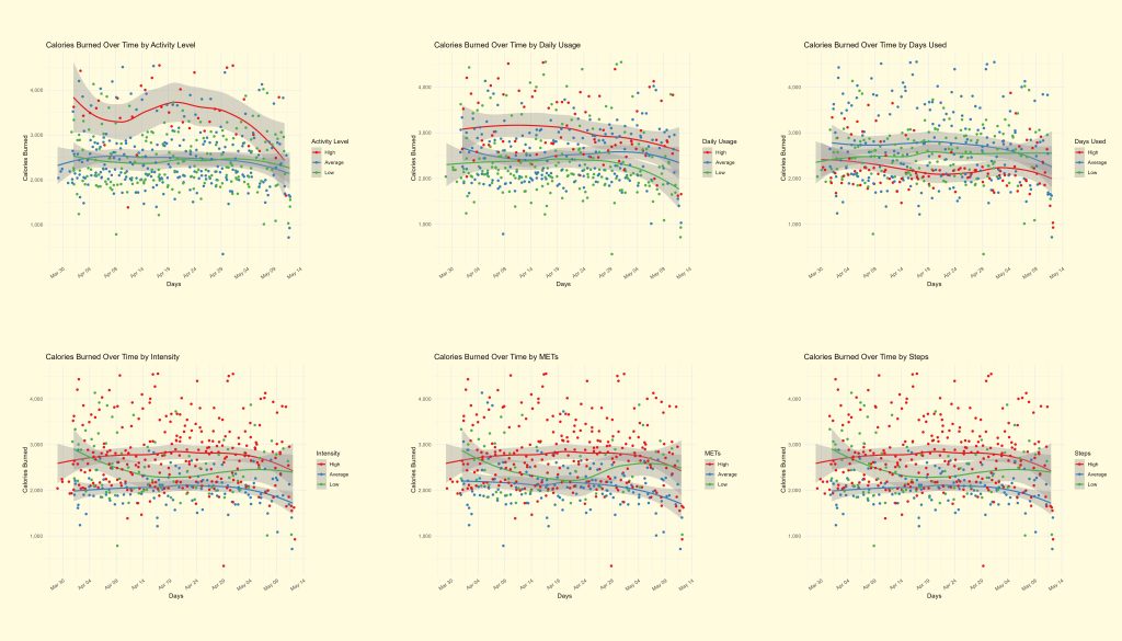
Looking at these charts, we can easily see that only the activity level grouping shows interesting trends. With this information, we can look at activity level metrics in more detail.
Additionally, we see that while the most active people burned more calories daily on average, this tapered off as time went on, showing how they likely need to change their workout habits to continue to see benefits.
Now, let’s see how the different activity levels’ heart rates look over time, as well as on average throughout the data collection period:
The code for the remaining charts can all be found in the appendix.
Now, let’s see how the different activity levels’ heart rates look over time, as well as on average throughout the data collection period:
The code for the remaining charts can all be found in the appendix.
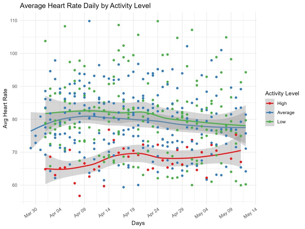
Over time, we can see that the most active people also have lower average heart rates, but again, these start to increase over time, as they seem to have adjusted to the more intense activity.
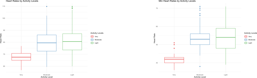
With these box plots, we can look at the average heart rates and minimum heart rates (considered as the average resting heart rate) by activity levels. It’s clear that more active people have healthier heart rates, rather significantly lower than average and low level activity participants. This will be interesting for our recommendations later.
It’s important to look at the other metrics to see if there are any other patterns around heart rates: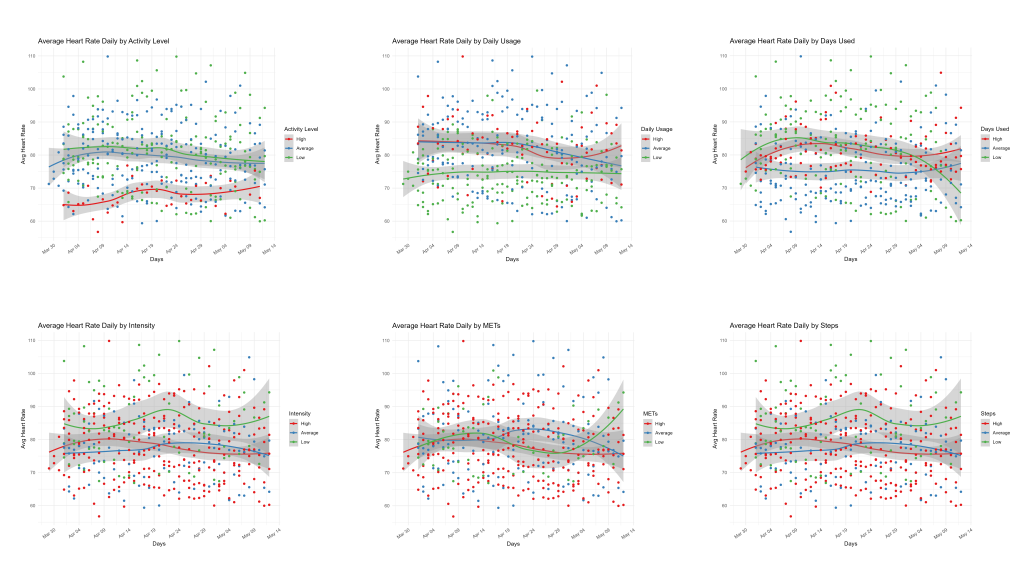
With these plots, we see again the clear trend by activity levels. The confidence intervals show us that most of the other groupings aren't very indicative of trends. However, there does seem to be some unusual correlations between usage of apps/devices with heart rates, something we didn't see in the calorie chart
We'll be looking at usage metrics next, but for now, we should focus our recommendations on heart rates, calories, and activity levels.
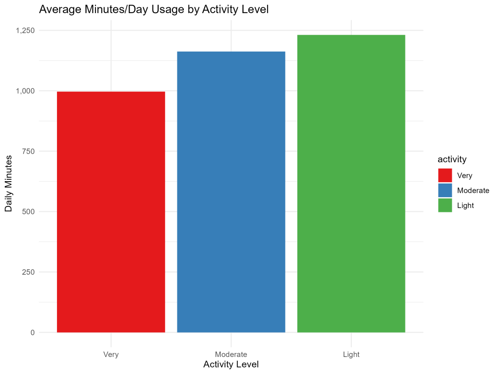
Now, we want to look at tracker usage patterns with the users. We can use bar charts to see how activity levels add to the picture, if at all.
We'll be looking at usage metrics next, but for now, we should focus our recommendations on heart rates, calories, and activity levels.
Now, we want to look at tracker usage patterns with the users. We can use bar charts to see how activity levels add to the picture, if at all.
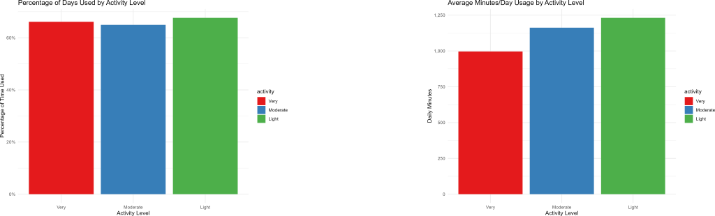
It’s very interesting to see that as activity levels drop, app/device usage increases. This will be part of our analysis as well.
On the other hand, the amount of days people logged data during the trial period is relatively identical for all fitness levels, so there isn’t much to learn from this.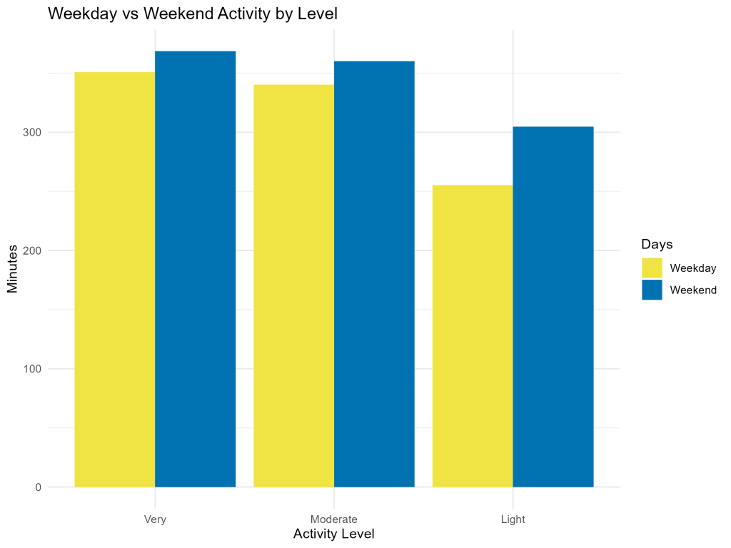
This last bar chart shows that in all groups, weekend activity was greater than weekday activity. However, it’s notable that low activity users saw a much greater difference between weekday and weekend activity time.
This is likely to factor into the analysis as well.
All code for the phases 3 and 4 can be seen in the appendix.
This is likely to factor into the analysis as well.
All code for the phases 3 and 4 can be seen in the appendix.
Phase V - Share
Based on the analysis, these charts paint the most interesting picture of how people use their devices, and the benefits they receive from their activity levels, and would be used in our presentation to Bellabeat's marketing team with the notes provided below them: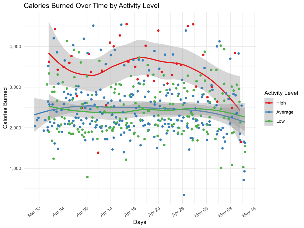
We see that high activity users have healthier heart rates, more calorie burn, and the most balanced usage for weekdays and weekends, but the least amount of usage daily. Over time, the health benefits seem to wane, showcasing the need for changing behaviors to get results.
Conversely, low activity users do not see the same health benefits, yet they use their devices more than the other groups. However, they have lower activity on the weekdays by far than either other group.
Notably, the points off the trendlines seem to show that these findings are even stronger with large parts of each activity level.
Phase VI - Act
Looking at these two groups of people in particular (noting that the moderate level users will likely respond to one of the campaigns), we can make the following recommendations for Bellabeat marketing:- High activity users - They would benefit greatly from the subscription service, as having someone guide their fitness over time would help them avoid plateaus and get them using the device and app more to help them with their health. It is recommended to market the subscription service to more athletic people, who may not immediately see the benefits of fitness trackers, but with this data to back it up, they could be brought into the Bellabeat subscription family.
- Low activity users - They show a need for motivation to be more active during the weekdays especially. The Leaf or Time devices paired with app notifications would help remind them to move more, and should be paired with weekly charts of their progress for encouragement. From a marketing perspective, advertising approachable fitness plans in the app, along with the clear ease of use of Leaf and Time, should drive more sales to the people who could see great progress with just a small push.
- Focusing on heart rate and calorie burn when marketing to potential customers will be great for all activity levels, as seeing something beyond weight loss will help them count smaller, earlier, successes, and keep them in the app for the long term.

About Me
Data analyst with 5+ years experience in analytics, databases, programming, and visualizations with expertise in Python, SQL, VBA, GAS, Excel, Sheets, Tableau, and R. Actively seeking work within a dynamic team.